6.2. Probability Distribution

Definition (probability distribution):

A function describes how probabilities are distributed over the values of the random variable.

1. Discrete Random Variable:

Example 1 (continue):

Suppose the probability for the outcomes in the gamble example is

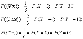
Let be some function corresponding to the probability of the gambling outcomes for

random variable X, defined as

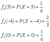
is referred as the probability distribution of random variable X.

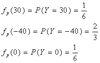
Similarly, the probability distribution of random variable Y is

Required conditions for a discrete probability distribution:

Let 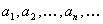be all the possible values of the discrete random variable X. Then,

the required conditions for to be the discrete probability distribution for X are

(a)

(b)

Example 1 (continue):

In the gambling example, is a discrete probability distribution for the

random variable X since

(a) .

(b) .

Similarly, is also a discrete probability distribution for the random variable Y.

Note: the discrete probability distribution describes the probability of a discrete

random variable at different values.

2. Continuous Random Variable:

For a continuous random variable, it is impossible to assign a probability to every

numerical value since there are uncountable number of values in an interval. Instead,

the probability can be assigned to a small interval. The probability density function can

describe how the probability distributes in the small interval.

Example 2 (continue):

In the delay flight time example, suppose the probability of being late within 0.5 hours is

two times of the one of being late more than 0.5 hour, i.e.,

.

Then, the probability density function for the random variable Z is

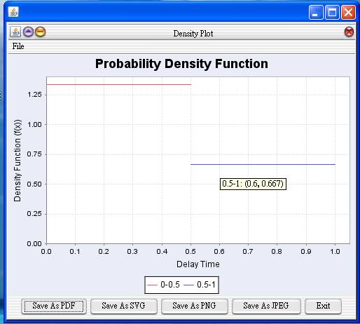
The area corresponding to the interval is the probability of the random variable Z taking values

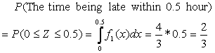
in this interval. For example, the probability of the flight time being late within 0.5 hour

(the random variable Z taking value in the interval [0,0.5]). is

.

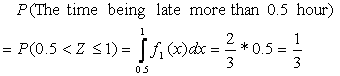
Similarly, the probability of the flight time being late more than 0.5 hour (the random variable Z

taking value in the interval (0.5,1]). is

.

On the other hand, If the probability of being late within 0.5 hours is the same as the one of

being late more than 0.5 hour, i.e.,

,

then, the probability density function for the random variable Z is

Note that the probability density function corresponds to the probability of the random variable

taking values in some interval. However, the probability density function evaluated at some

value could be larger than 1. It can not be used to describe the probability of the random

variable Z taking this value.

Required conditions for a continuous probability density:

Let the continuous random variable Z taking values in [a,b]. Then, the required conditions for

to be the continuous probability density for Z are

(a)

(b)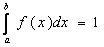

Note:

.

That is, the area under the graph of corresponding to a given interval is the probability

of the random variable Z taking value in this interval.

Example 2 (continue):

In the flight time example, is a continuous probability density for the random variable

Z since

(a) .

(b) .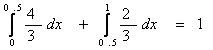

Similarly, is also a continuous probability density for the random variable Z.

JavaStatSoft:

Probability density:

Statistics -> Probability -> Probability Functions -> Probability Density Function (PDF)

Probability density:

Statistics -> Probability -> Probability Functions -> Cumulative Distribution Function (CDF)

Percentile (or Quantile):

Statistics -> Probability -> Probability Functions -> Percentile Function